QSAR
The QSAR tool covers model building, review and prediction. Model building comprises four steps: data selection, train/test splitting, descriptor choice and algorithm selection. The QSAR Analysis view in the top catalog allows users to inspect the model metrics and prediction results.
Typical workflow
- 01 Data Choose endpoint and task
- 02 Split Define training and test sets
- 03 Descriptors Choose molecular features
- 04 Methods Select algorithms and train
After reviewing a model, use QSAR → Predict to score ligands and inspect their predictions in QSAR Analysis → Result analysis.
0. Import ligands and activities
Before building a model, import the molecular structures and their measured activities through the Ligands catalog. For a CSV, include a SMILES column and one or more numeric/categorical activity columns, with each row containing a compound and its measurements.
For example, a CSV can use the following layout. These five entries are from the MoleculeNet BACE dataset:
| smiles | name | pIC50 | BACE_Class |
|---|---|---|---|
n1ccc2c(cccc2)c1N |
BACE_202 | 3 | 0 |
n1c2c(ccc1N)cccc2 |
BACE_203 | 3 | 0 |
O=C1NC(=NC(=C1)CCC)N |
BACE_205 | 2.6989701 | 0 |
O=C(NC1CCCCC1)CCc1cc2cc(ccc2nc1N)-c1ccccc1C |
BACE_89 | 7.1307683 | 1 |
Fc1ccc(NC(=O)c2ncc(cc2)C#N)cc1[C@]1(N=C(OCC1)N)C |
BACE_78 | 7.2923999 | 1 |
Here, smiles supplies the molecular structure and name identifies the
compound. pIC50 is a continuous endpoint for regression; BACE_Class
contains binary labels for classification (0 = inactive, 1 = active).
Your file can contain either or both endpoint types, using column names that
describe your measurements. Save the data as a CSV with a header row, and
select the activity columns during import as described below.
- Open Ligands → Import..., select Add files, and choose the input file.
-
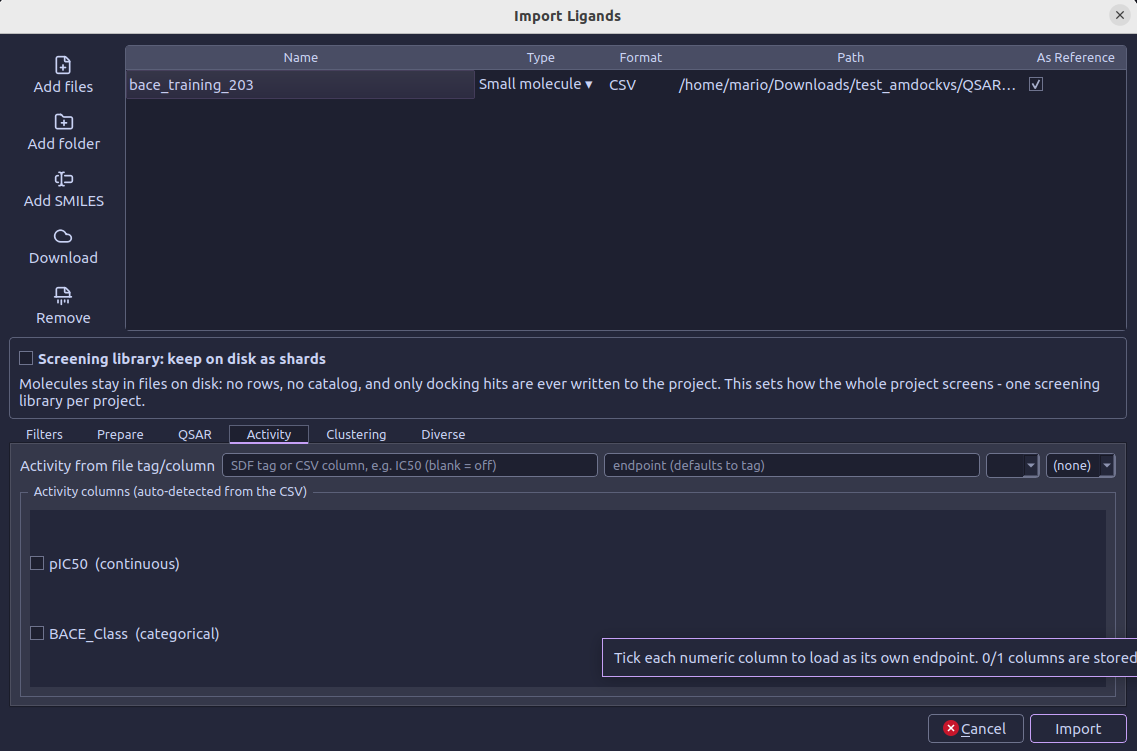
Tick As Reference for each file containing activity measurements. This enables the Activity tab below the file table and allows its measurements to be imported. Reference compounds are stored as project rows, even when screening-library sharding is enabled. Include both active and inactive compounds; the reference mark does not indicate an activity class.
-
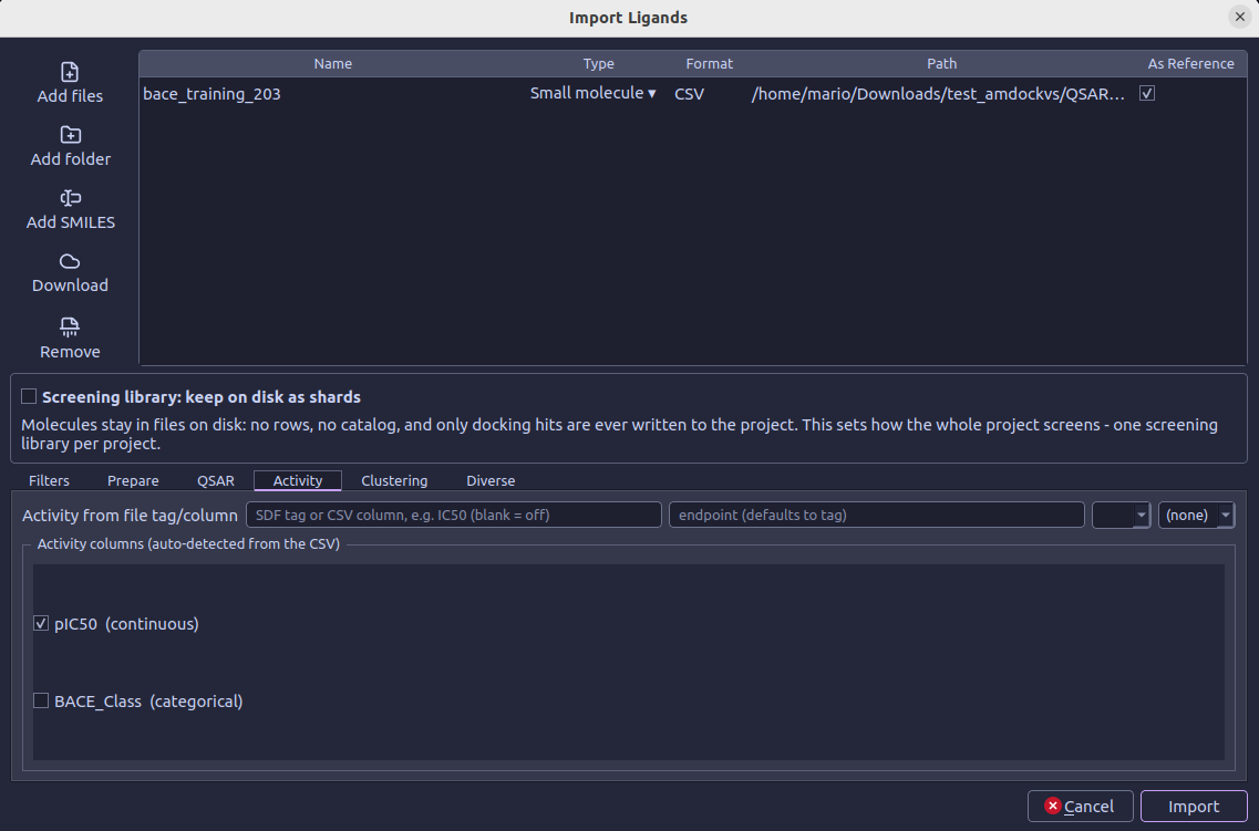
Activity should open automatically when the user ticks as Reference. Under Activity columns (auto-detected from the CSV), tick the columns to import as endpoints. For example, select pIC50 (continuous) for regression and BACE_Class (categorical) for binary classification. The detected columns are unchecked by default; tick the required measurements explicitly and leave unrelated numeric columns unchecked.
-
When using the detected-column checkboxes, leave Activity from file tag/column blank. For values already expressed as pIC50, leave the transform at (none); do not convert them again or assign concentration units such as nM. To import a single SDF property or table column instead, enter its name under Activity from file tag/column and configure its endpoint, unit and transform as needed.
-
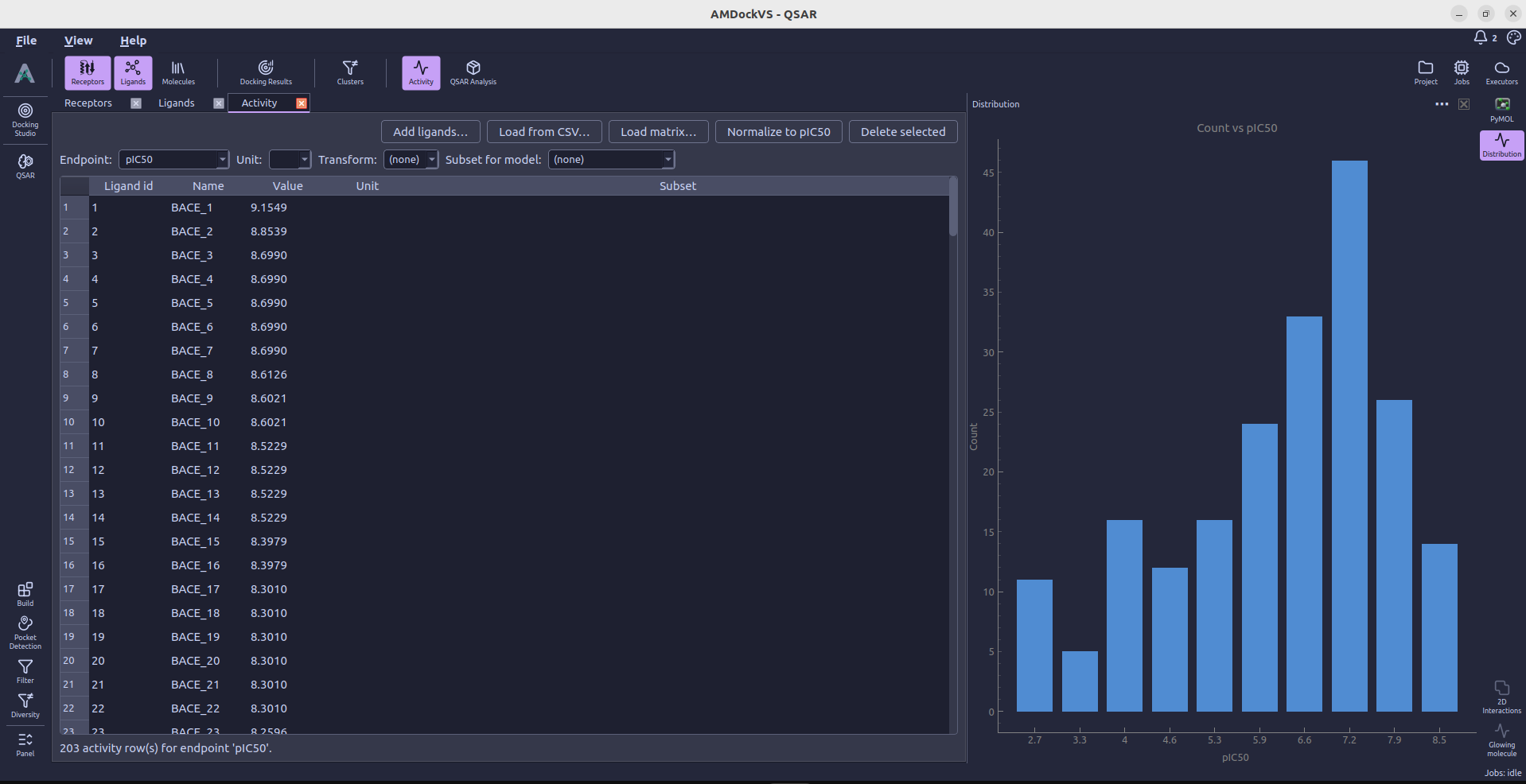
Select Import and follow progress in the Jobs monitor. Once the job finishes, open Activity from the top toolbar and check that the endpoints and measurements are present.
As Reference and activity columns are both required
For a CSV imported through the column checkboxes, marking the file As Reference enables activity import, but does not select any columns. Without selecting the activity columns, the molecules can be imported without the measurements needed to train a model.
See Ligands for more detail on activity import. Once the data are available, open QSAR → Build to follow the four model setup steps below.
1. Choose data
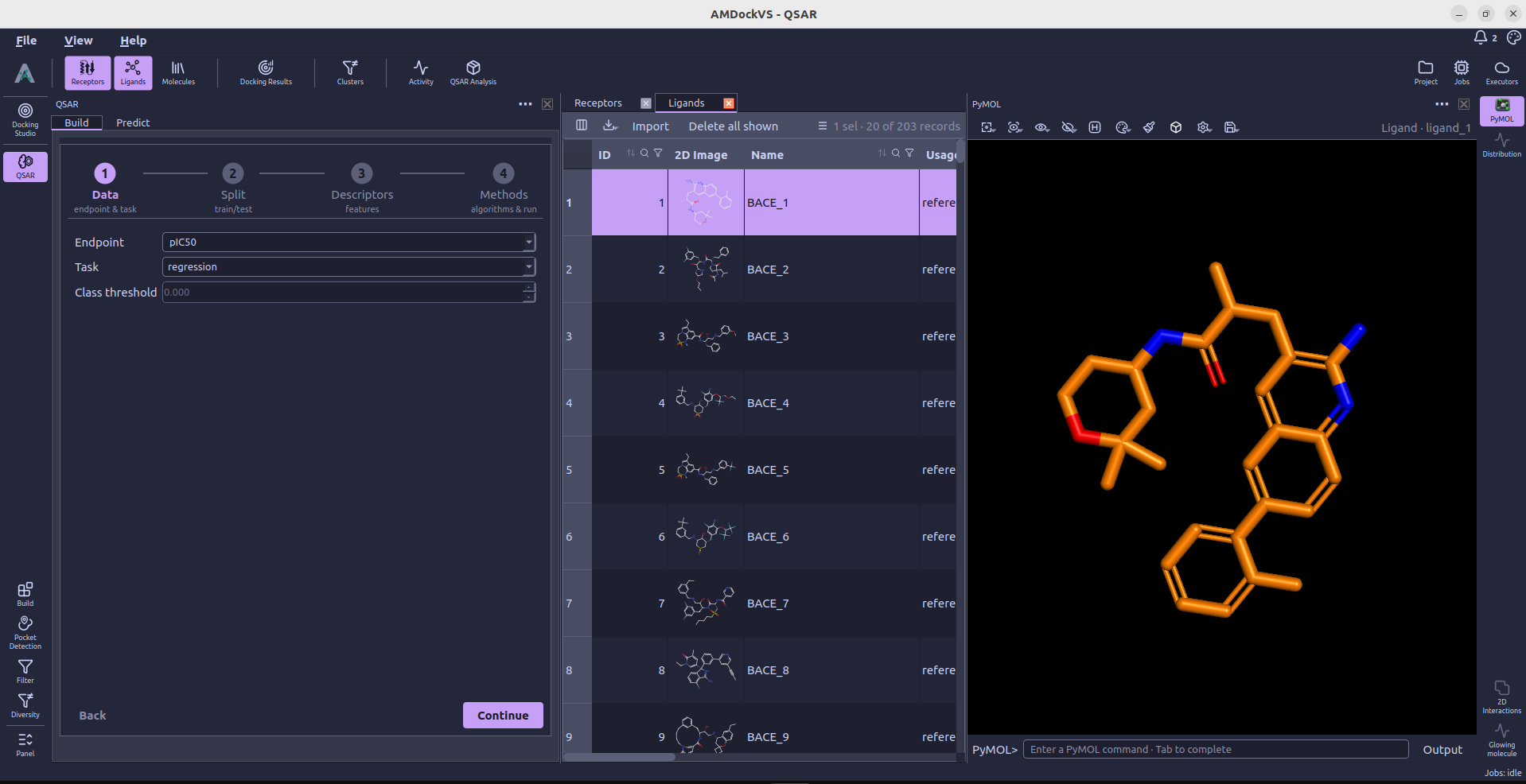
In Data, choose the activity endpoint (target variable) and set the task to regression or classification. A continuous endpoint can be converted to classes with a threshold; categorical endpoint labels are used directly.
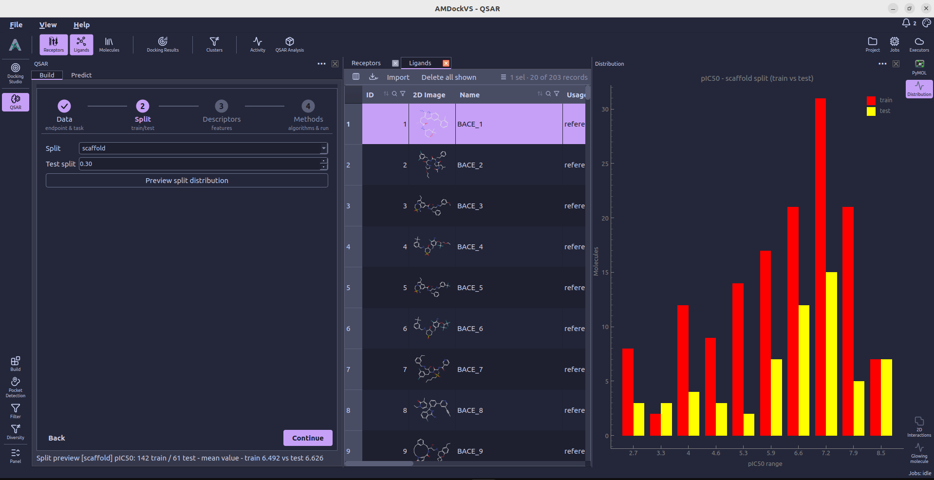
2. Split the data
In Split, choose a holdout test fraction and a splitting method. The available methods include random, stratified, scaffold, Butina and MaxMin splits. Use Preview split distribution to inspect the train and test distribution before training.
3. Choose descriptors
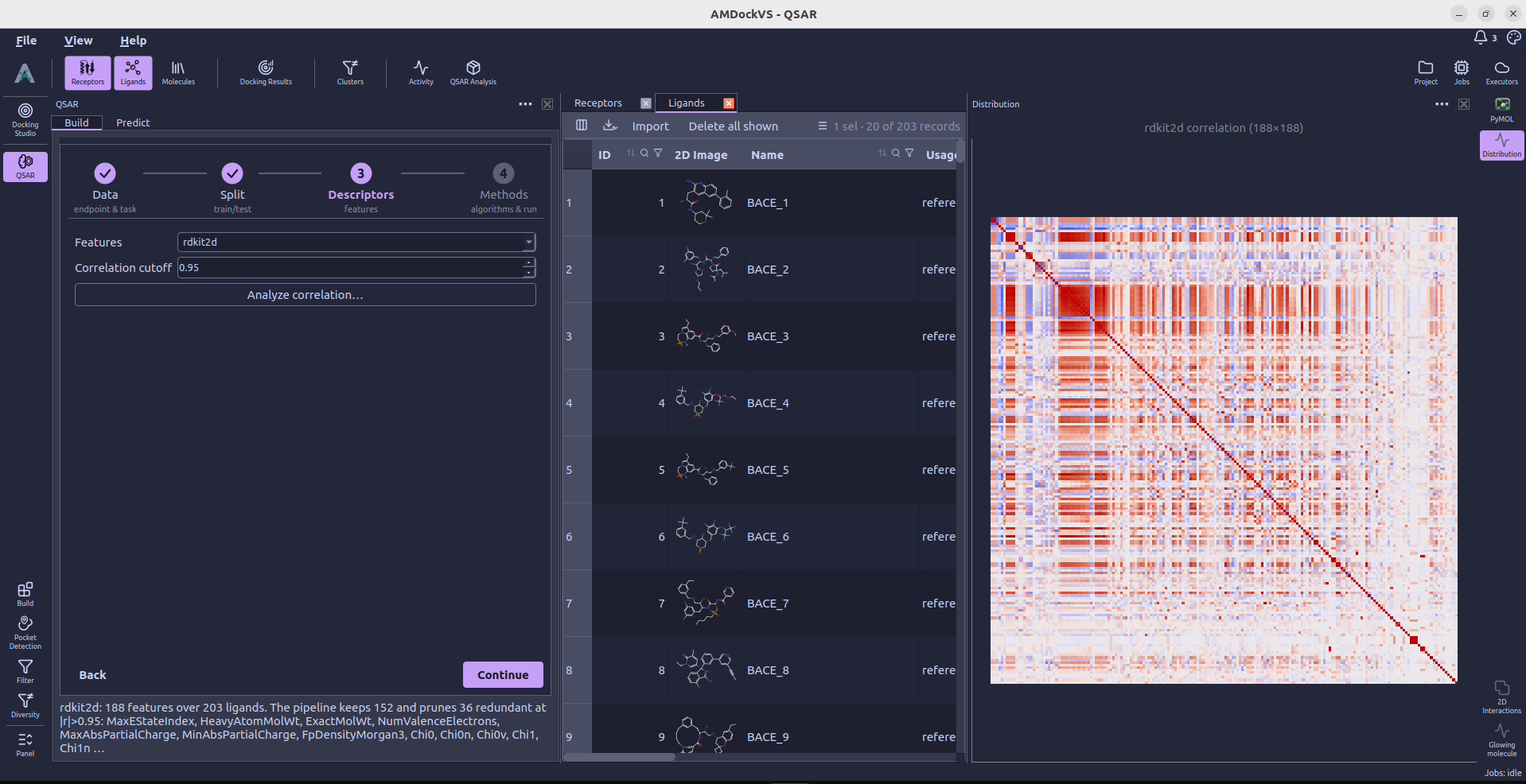
In Descriptors, choose RDKit 2D descriptors or ECFP4 fingerprints. RDKit descriptors can be pruned by a correlation cutoff; ECFP4 exposes the fingerprint radius and bit count. Missing features are calculated as part of the training jobs.
4. Select methods and train
In Methods, select one or more supported algorithms to compare, then set cross-validation folds and optional y-scramble runs. Select Train to submit the model job.
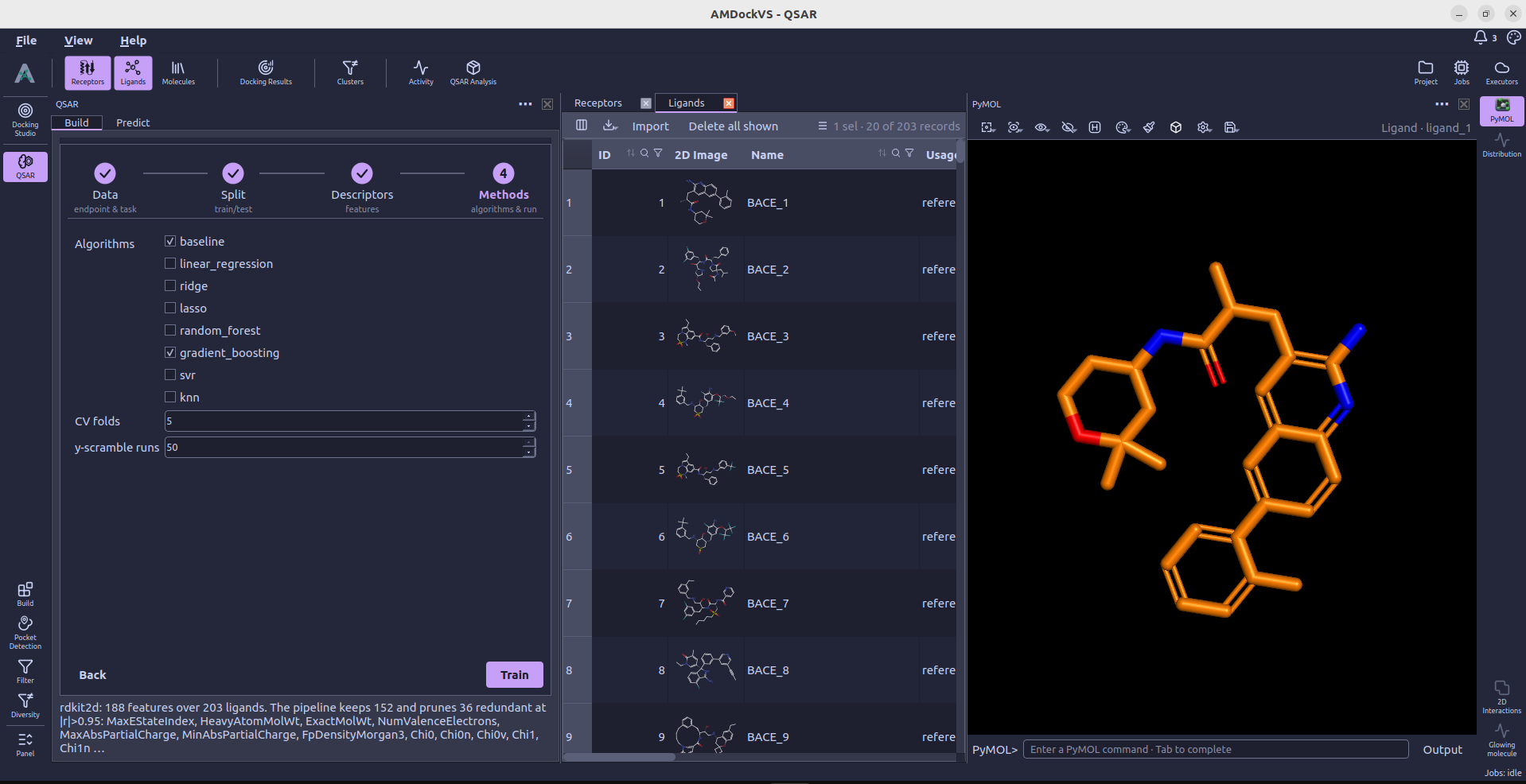
Training jobs appear in the Jobs monitor. After submission, AMDockVS opens QSAR Analysis → Model analysis, where the models become available as training completes.
Analyze models
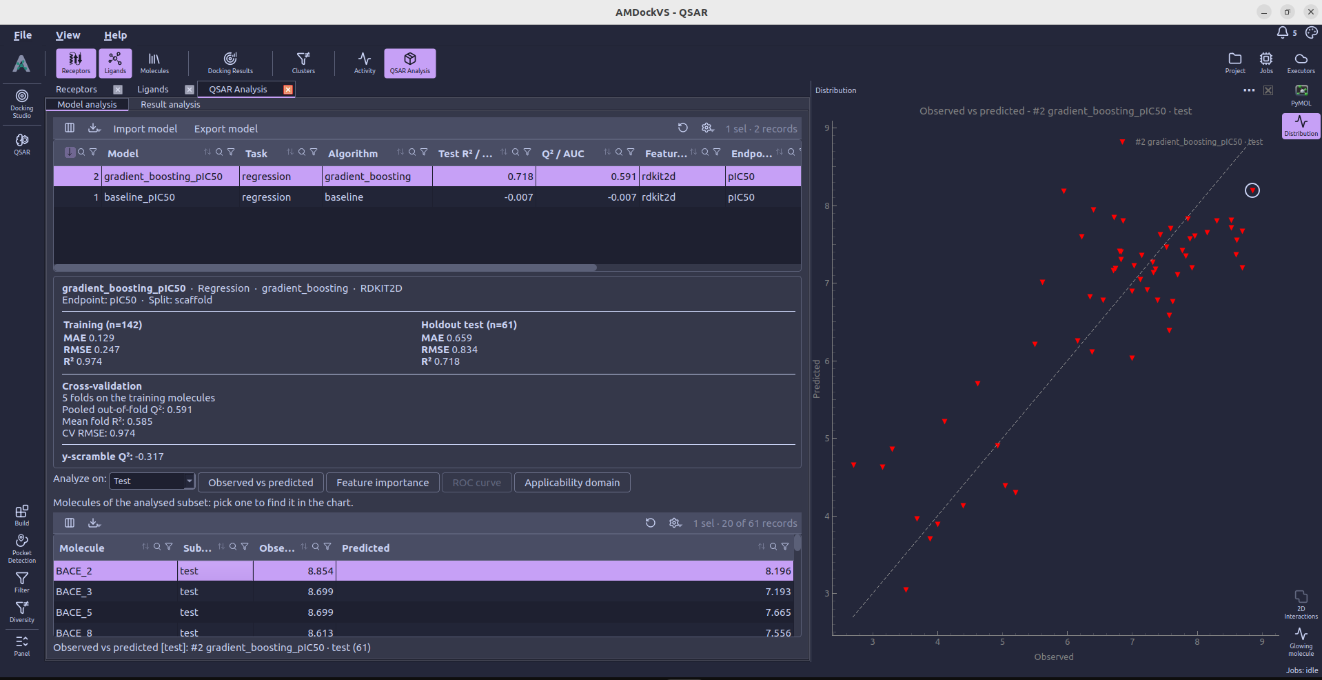
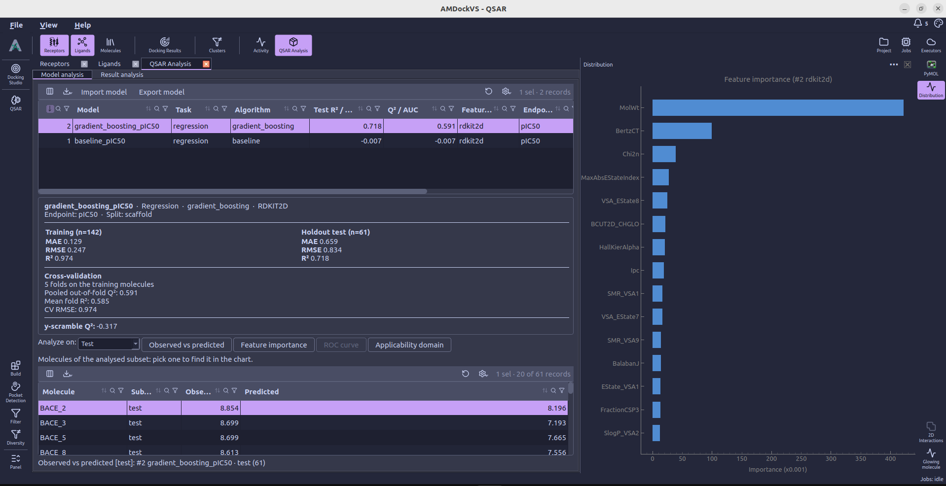
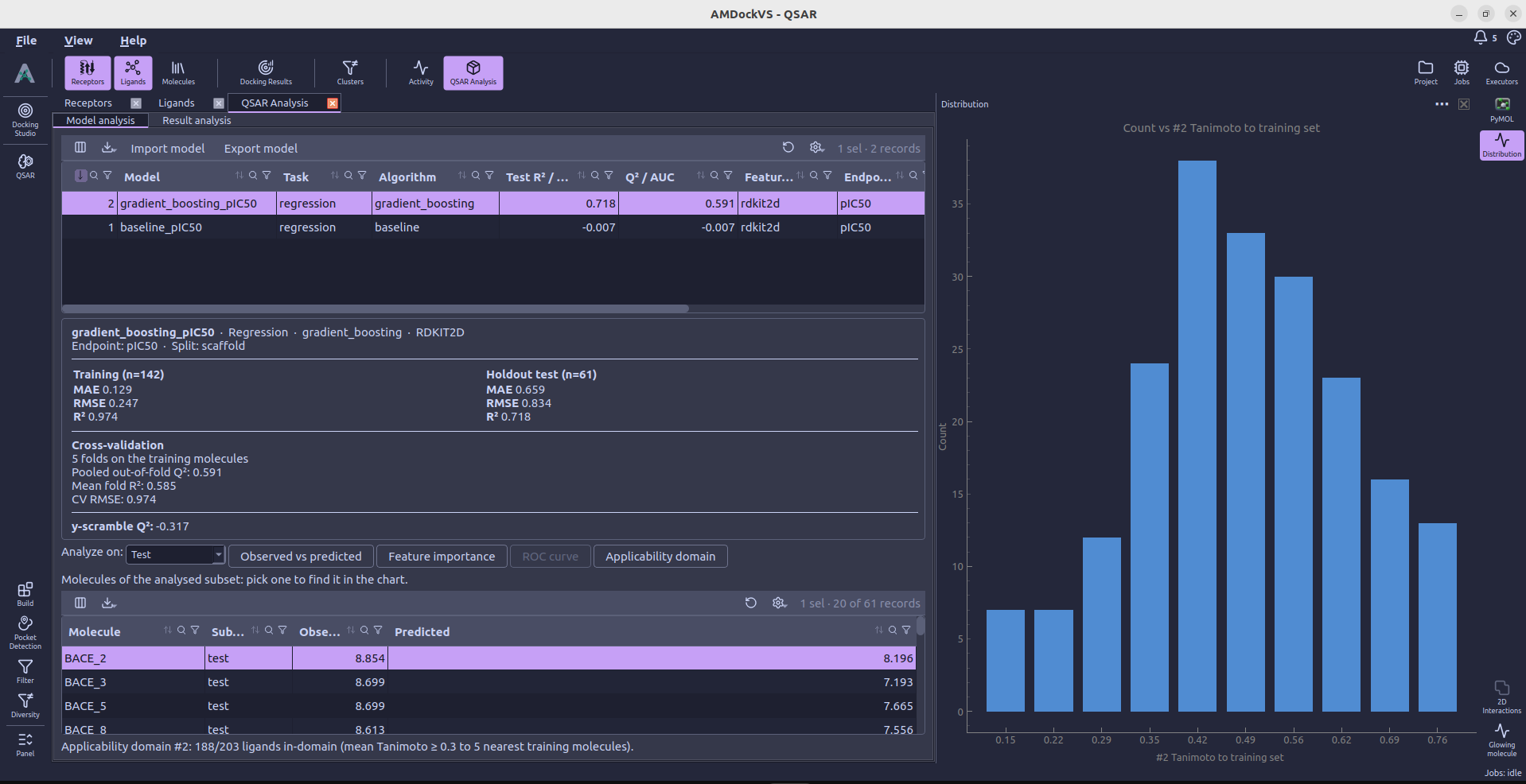
Model analysis lists trained models and summarizes their task, algorithm, feature type, endpoint, split and reported metrics. Select a model to review its training, holdout-test and cross-validation results. Depending on task and model type, the analysis tools include observed-versus-predicted plots, ROC analysis, feature importance and applicability-domain checks. Selecting a molecule in the model’s analyzed subset links it to the corresponding point in the chart.
Predict
Under construction
The QSAR prediction workflow is under construction. The following description is a placeholder for the final workflow.
In QSAR → Predict, tick one or more saved models and choose how to score the project’s ligands. Predict all ligands submits prediction jobs for the selected models. For a screening library stored as shards, use Predict shards; scores remain associated with the shards until you choose Promote top... to add the best-scoring molecules from one model as ligand rows.
After prediction, the application opens QSAR Analysis → Result analysis for that model. Predictions can be reviewed in the results table and filtered by selecting a top N or a value cutoff. Use as selection applies the kept ligands as the global ligand selection. Exclude the rest marks the other scored ligands as excluded; they remain in the project and can be recovered through Filter.
Result analysis shows a selected model’s predictions, confidence and applicability-domain similarity for scored ligands. Selecting a row can highlight that molecule in the 3D viewer when the model uses ECFP4 fingerprints. The applicability-domain value is the mean Tanimoto similarity to the model’s nearest training molecules; a low value flags a prediction as outside the configured domain threshold.
The programmatic interface for endpoints, model training and prediction is documented in the QSAR section of the API guide.